Week 1 Part 2 - Pre-training and Scaling Laws

These notes were developed using lectures/material/transcripts from the DeepLearning.AI & AWS - Generative AI with Large Language Models course

Notes #

• Pre-training Large Language Models
  • Stage 1 of Generative AI Project Lifecycle - Select
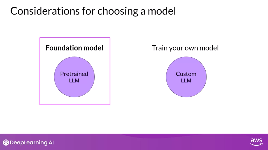
    • Work with an existing Foundation model or train your own model
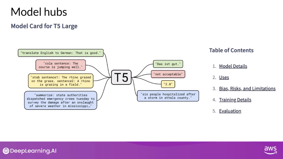
  • Model cards - model details, uses, bias, risks, limitations, training details and evaluation
  • Model Architectures and Pre-training Objectives
    • LLMs encode a deep statistical representation of language
    • The model’s pre-training phase - the model learns from vast amounts of unstructured textual data (petabytes of text)
    • In this self-supervised learning step, the model internalizes the patterns and structures present in the language
    • Transformer Variants
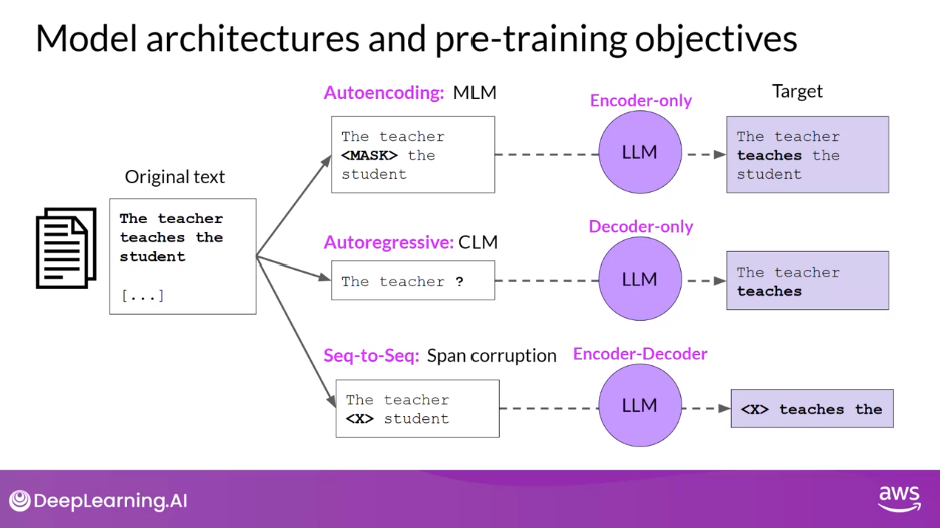
      • Autoencoding (encoder only) models - trained using Masked Language Modeling (MLM), denoising objective
        • Build bi-directional representations of the input sequence, meaning that the model has an understanding of the full context of a token and not just of the words that come before
        • Tasks: Sentiment Analysis, Named Entity Recognition (NER), Sentence/Word/Token Classification
        • Models: BERT, RoBERTa
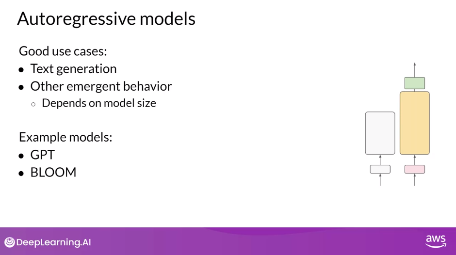
      • Autoregressive (decoder only) models - trained using Causal Language Modeling (CLM)
        • Mask the input sequence and can only see the input tokens leading up to the token in question, the model has no knowledge of the end of the sentence. The context is unidirectional
        • By learning to predict the next token from a vast number of examples, the model builds up a statistical representation of language
        • Tasks: Text Generation, Emergent Abilities (Zero Shot Inference, etc.)
        • Models: GPT, BLOOM
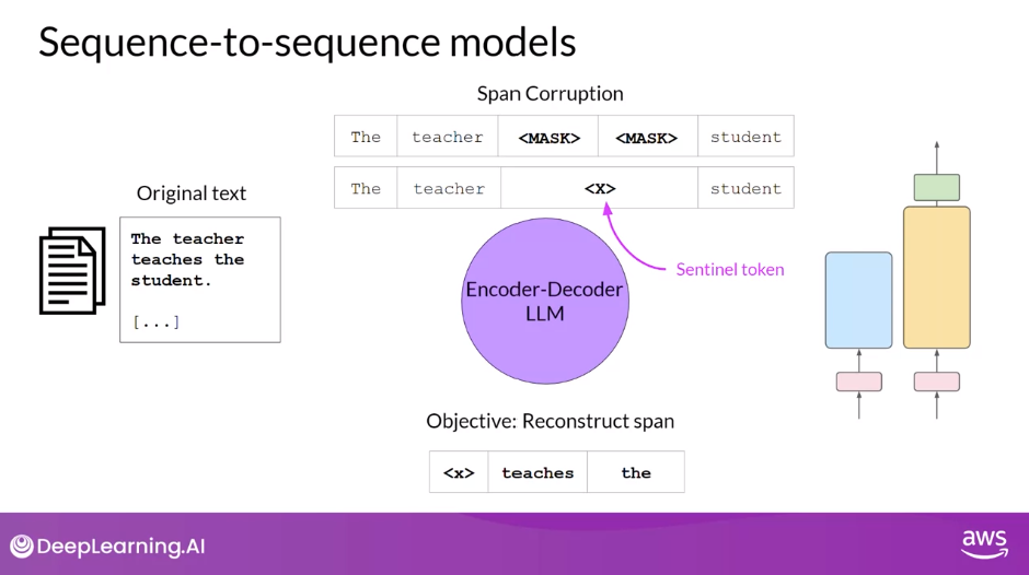
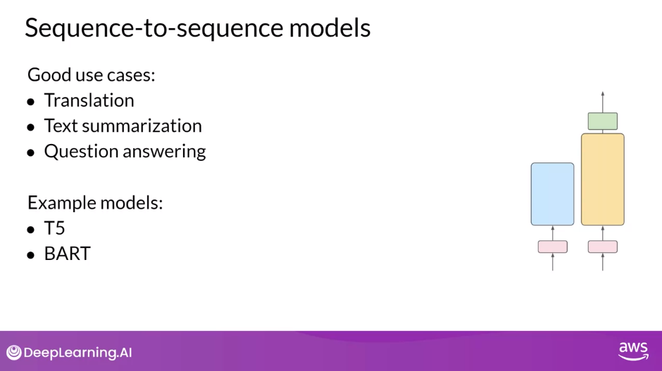
      • Sequence-to-Sequence (encoder-decoder) models
        • Exact details of the pre-training objective vary from model to model
        • Tasks: Translation, Text Summarization, and Question Answering
        • Models: T5, BART
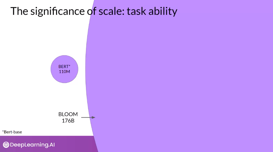
    • The Significance of Scale: Task Ability
      • The larger a model, the more likely it is to work as you needed to without additional in-context learning or further training
• Computational Challenges of Training LLMs
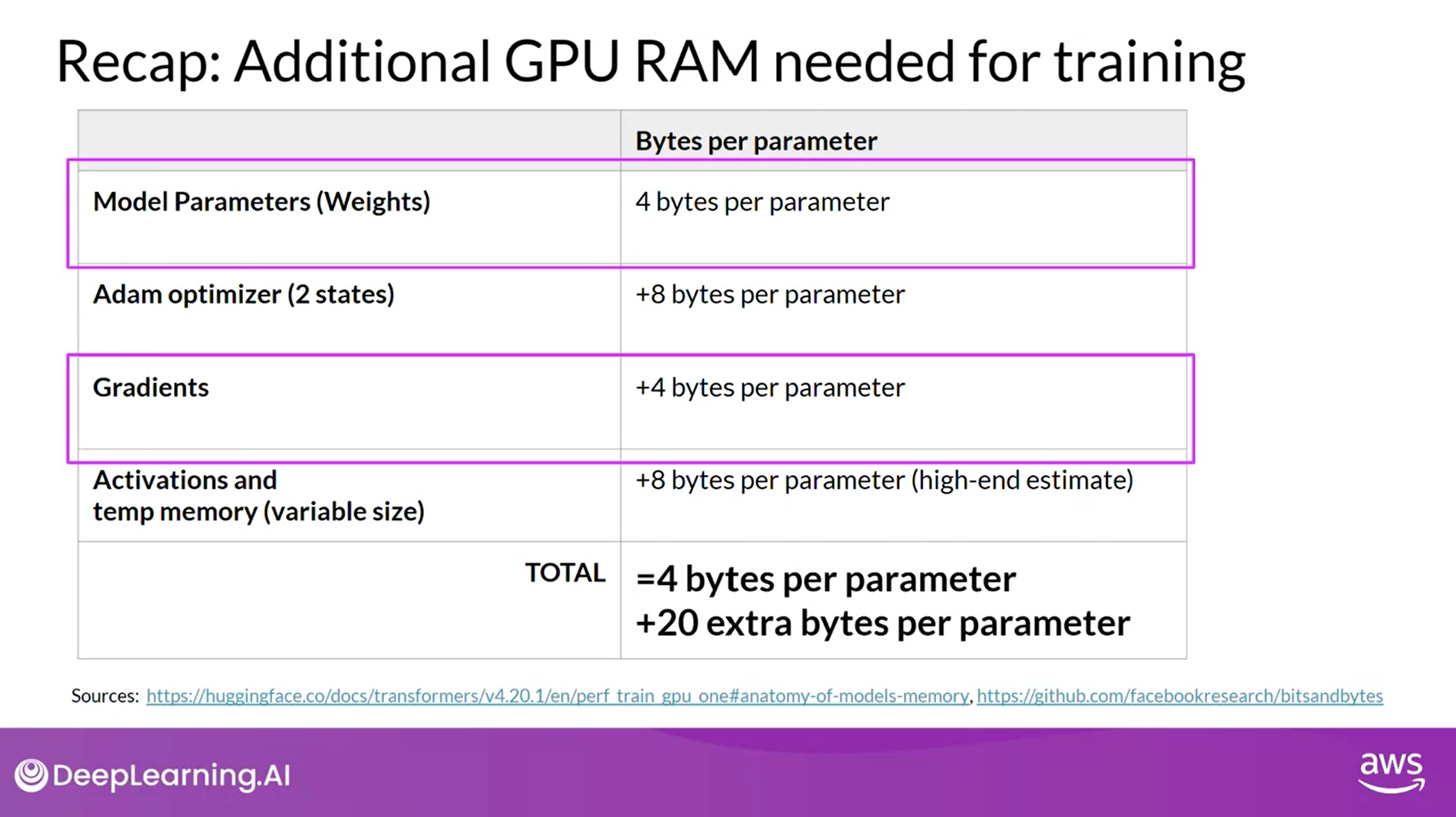
  • Challenges: OutOfMemoryError - CUDA out of memory
  • Require sufficient memory to store all this:
    1. Weights: 4 bytes per parameter
    2. Two Adam optimizer states: 8 bytes per parameter
    3. Gradients: 4 bytes per parameter
    4. Activations and Temporary variables needed by your functions: 8 bytes per parameter
    • Total: 4 bytes per parameter + 20 extra bytes per parameter
  • Quantization - reduce the memory requirement by reducing their precision
    • Memory to store a number
      • Bits
      • Exponent
      • Fraction (referred to as Mantissa)
    • Data Types
      • FP32: 4 bytes of memory
      • FP16: 2 bytes of memory
      • BFLOAT16: 2 bytes of memory
        • Hybrid between half precision FP16 and full precision FP32
        • Downside: not well suited for integer calculations
      • INT8: 1 byte of memory
      • INT4
    • Quantization statistically projects the original 32-bit floating point numbers into a lower precision space, using scaling factors calculated based on the range of the original 32-bit floating point numbers
    • Quantization-Aware Training (QAT) learns the quantization scaling factors during training
    • Note: Quantization does not reduce the number of model parameters
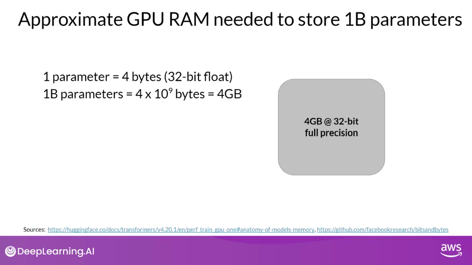
  • Approximate GPU RAM Needed to Store and Train 1B Parameters
    • Memory needed to store model: 4GB @32-bit full precision
      • 2GB @16-bit half precision
      • 1GB @8-bit precision
    • Memory needed to train model: 80GB @32-bit full precision
      • 40GB @16-bit half precision
      • 20GB @8-bit precision
    • 80GB is the maximum memory for the NVIDIA A100 GPU
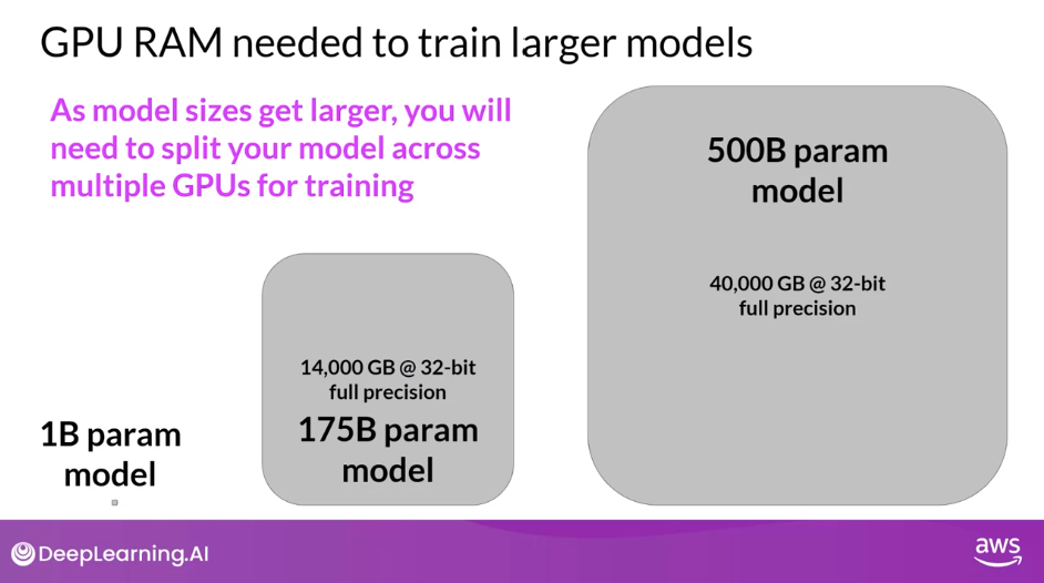
  • As the model sizes get larger, you will need to split your model across multiple GPUs for training
• Optional: Efficient Multi-GPU Compute Strategies
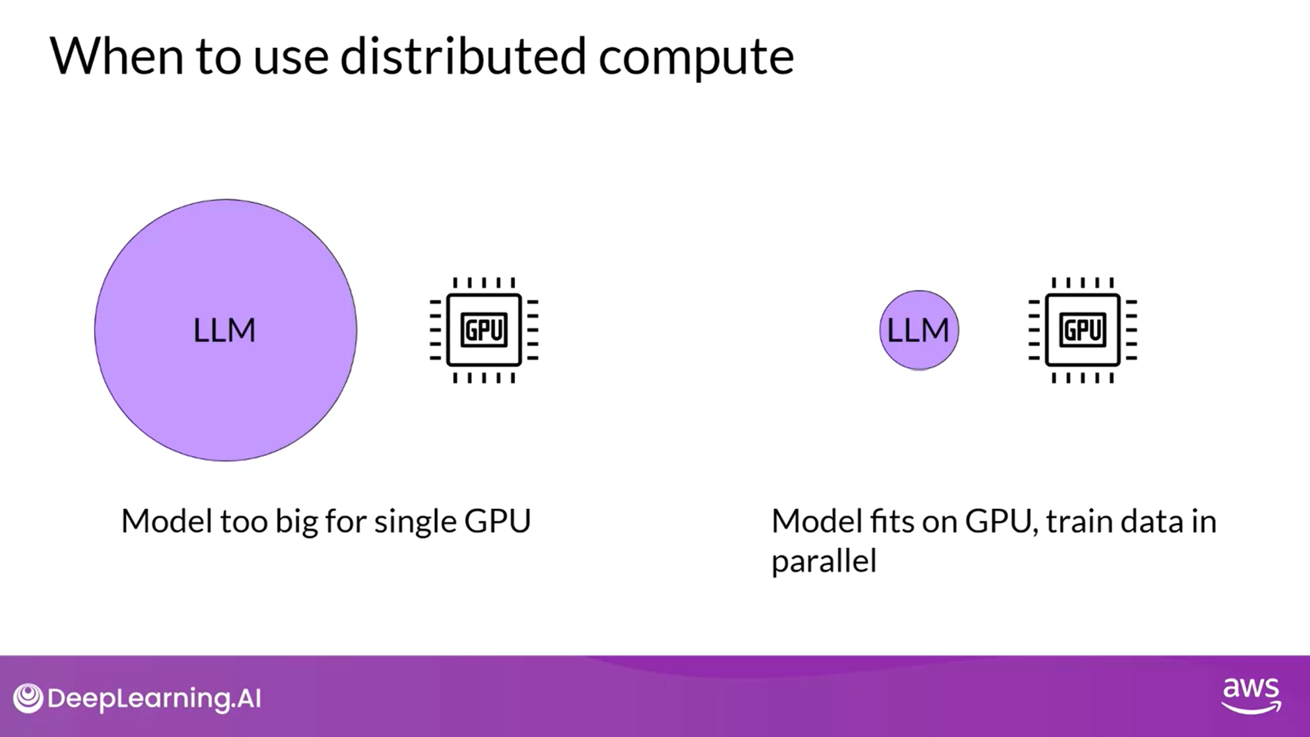
  • When to Use Distributed Compute
    1. Model too big for single GPU
    2. Model fits on GPU, train data in parallel
  • PyTorch Implementation
  • Distributed Data Parallel (DDP) - Model fits on a single GPU
    • Requires that your model weights and all of the additional parameters, gradients, and optimizer states that are needed for training, fit onto a single GPU
    • Copies your model onto each GPU and sends batches of data to each of the GPUs in parallel. Each data-set is processed in parallel and then a synchronization step combines the results of each GPU, which in turn updates the model on each GPU, which is always identical across chips
  • Fully Sharded Data Parallel (FSDP) - Model no longer fits on a single GPU
    • Model Sharding
    • FSDP is motivated by the “ZERO” paper - zero data overlap between GPUs
    • sharding factor - configure the level of sharding to manage the trade-off between performance and memory utilization
      • 1 = removes the sharding and replicated the full model similar to DDP
      • Maximum number of GPUs = full sharding
      • Anywhere in between = hybrid sharding
    • Can use FSDP for both small and large models and seamlessly scale your model training across multiple GPUs
• Scaling Laws and Compute-Optimal Models
  • To determine how big models need to be, learn about research that explore the relationship between
    • Model size
    • Training
    • Configuration
    • Performance
  • Scaling Choices for Pre-training
    • Goal: maximize the model’s performance of its learning objective, which is minimizing the loss when predicting tokens
    • Options to achieve better performance:
      1. Increasing the size of the dataset you train your model on
      2. Increasing the number of parameters in your model
    • Constraint: compute budget (number of GPUs, training time, cost)
  • Unit of Compute
    • “petaFLOP/s-day” = a measurement of the number of floating point operations performed at rate of 1 petaFLOP per second for one day
    • 1 petaFLOP corresponds to one quadrillion floating point operations per second
    • In the context of training transformers, 1 petaFLOP per second day is approximately equivalent to eight NVIDIA V100 GPUs, operating at full efficiency for one full day
  • Compute Budget vs Model Performance
    • Increase your compute budget to achieve better model performance
    • In practice however, the compute resources you have available for training will generally be a hard constraint set by factors such as
      • the hardware you have access to,
      • the time available for training and
      • the financial budget of the project
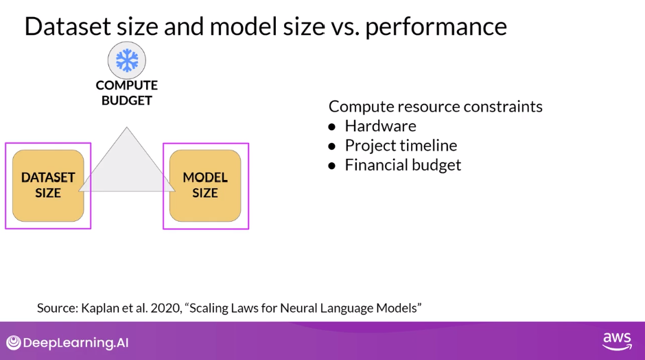
  • Dataset Size and Model Size vs Model Performance
    • As the volume of training data increases, the performance of the model continues to improve
    • As the model size increases in size, the test loss decreases indicating better performance
  • Chinchilla Paper: Training Compute-Optimal Large Language Models
    • Goal: to find the optimal number of parameters and volume of training data for a given compute budget
    • Findings
      1. Very large models may be over-parameterized and under-trained
      2. Smaller models trained on more data could perform as well as large model
  • Chinchilla Scaling Laws for Model and Dataset Size
    • The optimal training dataset size for a given model is about 20 times larger than the number of parameters in the model
    • The compute optimal Chinchilla model outperforms non-compute optimal models such as GPT-3 on a large range of downstream evaluation tasks
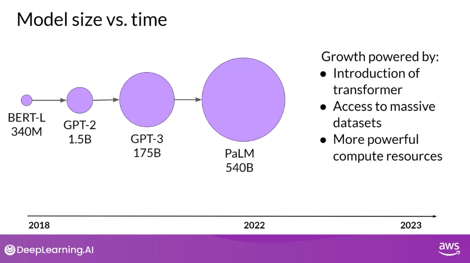
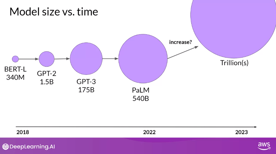
  • Model Size vs Time
    • Expect to see smaller models developed to achieve better results than larger models trained in a non-optimal way
• Pre-training for Domain Adaptation
  • Highly specialized domains: Law, Medical, Finance, Science
  • BloombergGPT: Domain Adaptation for Finance
    • Scaling Laws
• Reading: Domain-Specific Training: BloombergGPT
  • A large Decoder-only model
  • Pre-trained on finance data
  • Used Chinchilla Scaling Laws to guide the number of parameters in the model and volume of training data (tokens)

Pre-training Large Language Models #

Stage 1 of Generative AI Project Lifecycle - Select #

• Once you have scoped out your use case, and determined how you’ll need the LLM to work within your application, your next step is to select a model to work with. Your first choice will be to either work with an existing model, or train your own from scratch. There are specific circumstances where training your own model from scratch might be advantageous, and you’ll learn about those later in this lesson. In general, however, you’ll begin the process of developing your application using an existing foundation model

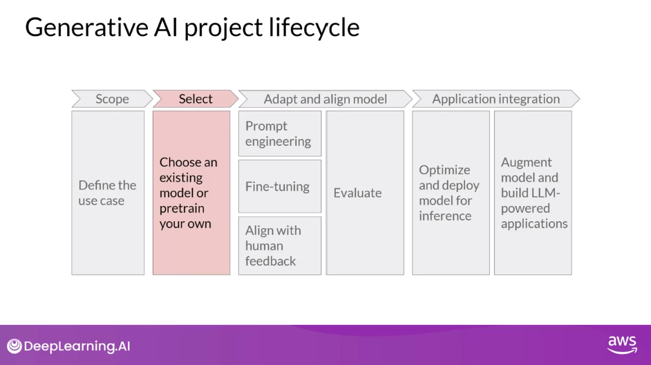
Model Cards #

• Describe important details including the best use cases for each model, how it was trained, and known limitations
• The exact model that you’d choose will depend on the details of the task you need to carry out
• Variance of the transformer model architecture are suited to different language tasks, largely because of differences in how the models are trained

Model Architectures and Pre-training Objectives #

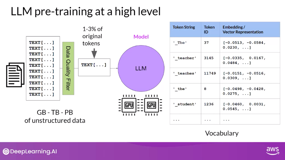
• Take a high-level look at the initial training process for LLMs
• This phase is often referred to as pre-training.
• As you saw in Lesson 1, LLMs encode a deep statistical representation of language.
• This understanding is developed during the model’s pre-training phase when the model learns from vast amounts of unstructured textual data.
• This can be gigabytes, terabytes, and even petabytes of text.
• This data is pulled from many sources, including scrapes off the Internet and corpora of texts that have been assembled specifically for training language models.
• In this self-supervised learning step, the model internalizes the patterns and structures present in the language.
• These patterns then enable the model to complete its training objective, which depends on the architecture of the model, as you’ll see shortly.
• During pre-training, the model weights get updated to minimize the loss of the training objective.
• The encoder generates an embedding or vector representation for each token.
• Pre-training also requires a large amount of compute and the use of GPUs.
• Note, when you scrape training data from public sites such as the Internet, you often need to process the data to increase quality, address bias, and remove other harmful content.
  • As a result of this data quality curation, often only 1-3% of tokens are used for pre-training.
  • You should consider this when you estimate how much data you need to collect if you decide to pre-train your own model

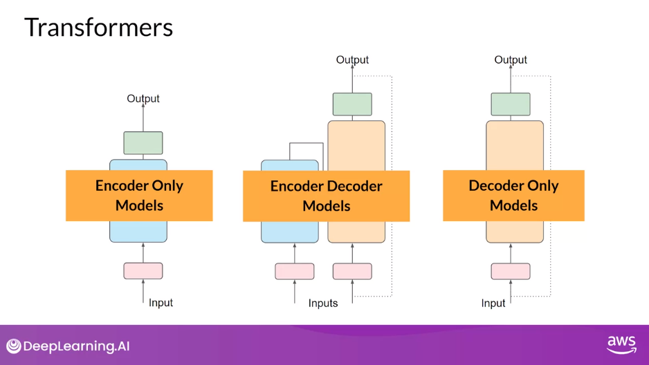
Transformer Variants #

1. Encoder Only Models
2. Encoder Decoder Models
3. Decoder Models

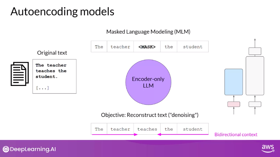
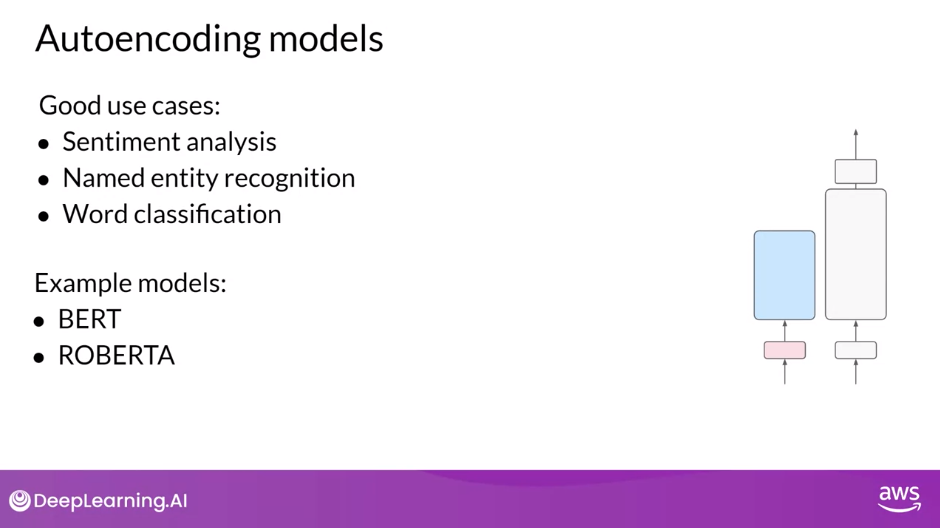
Autoencoding Models #

• Encoder-only models are also known as Autoencoding models, and they are pre-trained using masked language modeling. Here, tokens in the input sequence or randomly mask, and the training objective is to predict the mask tokens in order to reconstruct the original sentence. This is also called a denoising objective. Autoencoding models build bi-directional representations of the input sequence, meaning that the model has an understanding of the full context of a token and not just of the words that come before. Encoder-only models are ideally suited to task that benefit from this bi-directional contexts. You can use them to carry out sentence classification tasks, for example, sentiment analysis or token-level tasks like named entity recognition or word classification.
  • Some well-known examples of an autoencoder model are BERT and RoBERTa

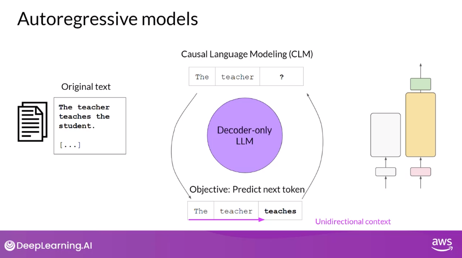
Autoregressive Models #

• let’s take a look at decoder-only or autoregressive models, which are pre-trained using causal language modeling. Here, the training objective is to predict the next token based on the previous sequence of tokens. Predicting the next token is sometimes called full language modeling by researchers. Decoder-based autoregressive models, mask the input sequence and can only see the input tokens leading up to the token in question. The model has no knowledge of the end of the sentence. The model then iterates over the input sequence one by one to predict the following token. In contrast to the encoder architecture, this means that the context is unidirectional. By learning to predict the next token from a vast number of examples, the model builds up a statistical representation of language. Models of this type make use of the decoder component off the original architecture without the encoder. Decoder-only models are often used for text generation, although larger decoder-only models show strong zero-shot inference abilities, and can often perform a range of tasks well.
  • Well known examples of decoder-based autoregressive models are GPT and BLOOM

Sequence-to-Sequence Models #

• The final variation of the transformer model is the sequence-to-sequence model that uses both the encoder and decoder parts off the original transformer architecture. The exact details of the pre-training objective vary from model to model. A popular sequence-to-sequence model T5, pre-trains the encoder using span corruption, which masks random sequences of input tokens. Those mass sequences are then replaced with a unique Sentinel token, shown here as x. Sentinel tokens are special tokens added to the vocabulary, but do not correspond to any actual word from the input text. The decoder is then tasked with reconstructing the mask token sequences auto-regressively. The output is the Sentinel token followed by the predicted tokens. You can use sequence-to-sequence models for translation, summarization, and question-answering. They are generally useful in cases where you have a body of texts as both input and output.
  • Besides T5, which you’ll use in the labs in this course, another well-known encoder-decoder model is BART

Model Summary #

• To summarize, here’s a quick comparison of the different model architectures and the targets off the pre-training objectives.
  • Autoencoding models are pre-trained using masked language modeling. They correspond to the encoder part of the original transformer architecture, and are often used with sentence classification or token classification.
  • Autoregressive models are pre-trained using causal language modeling. Models of this type make use of the decoder component of the original transformer architecture, and often used for text generation.
  • Sequence-to-sequence models use both the encoder and decoder part off the original transformer architecture. The exact details of the pre-training objective vary from model to model. The T5 model is pre-trained using span corruption. Sequence-to-sequence models are often used for translation, summarization, and question-answering.

The Significance of Scale: Task Ability #

• One additional thing to keep in mind is that larger models of any architecture are typically more capable of carrying out their tasks well.
• Researchers have found that the larger a model, the more likely it is to work as you needed to without additional in-context learning or further training

• This observed trend of increased model capability with size has driven the development of larger and larger models in recent years. This growth has been fueled by inflection points and research, such as
  • the introduction of the highly scalable transformer architecture,
  • access to massive amounts of data for training, and
  • the development of more powerful compute resources

• This steady increase in model size actually led some researchers to hypothesize the existence of a new Moore’s law for LLMs. Like them, you may be asking,
  • Can we just keep adding parameters to increase performance and make models smarter?
  • Where could this model growth lead?
• While this may sound great, it turns out that training these enormous models is difficult and very expensive, so much so that it may be infeasible to continuously train larger and larger models.

Computational Challenges of Training LLMs #

• OutOfMemoryError: CUDA out of memory.
• One of the most common issues you still counter when you try to train large language models is running out of memory.
• If you’ve ever tried training or even just loading your model on NVIDIA GPUs, this error message might look familiar.
• CUDA, short for Compute Unified Device Architecture, is a collection of libraries and tools developed for Nvidia GPUs.
• Libraries such as PyTorch and TensorFlow use CUDA to boost performance on matrix multiplication and other operations common to deep learning.
• You’ll encounter these out-of-memory issues because most LLMs are huge, and require a ton of memory to store and train all of their parameters.

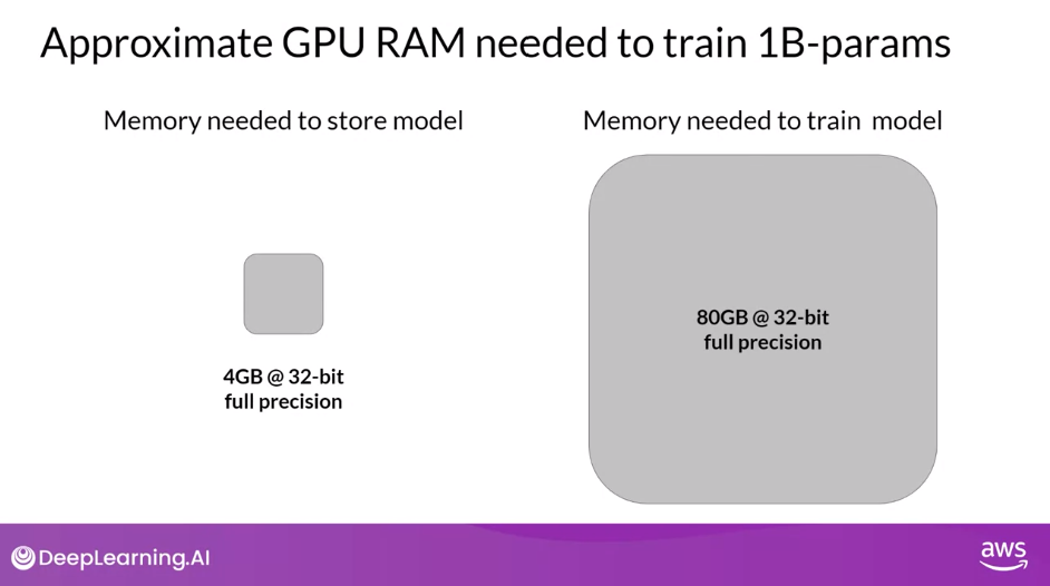
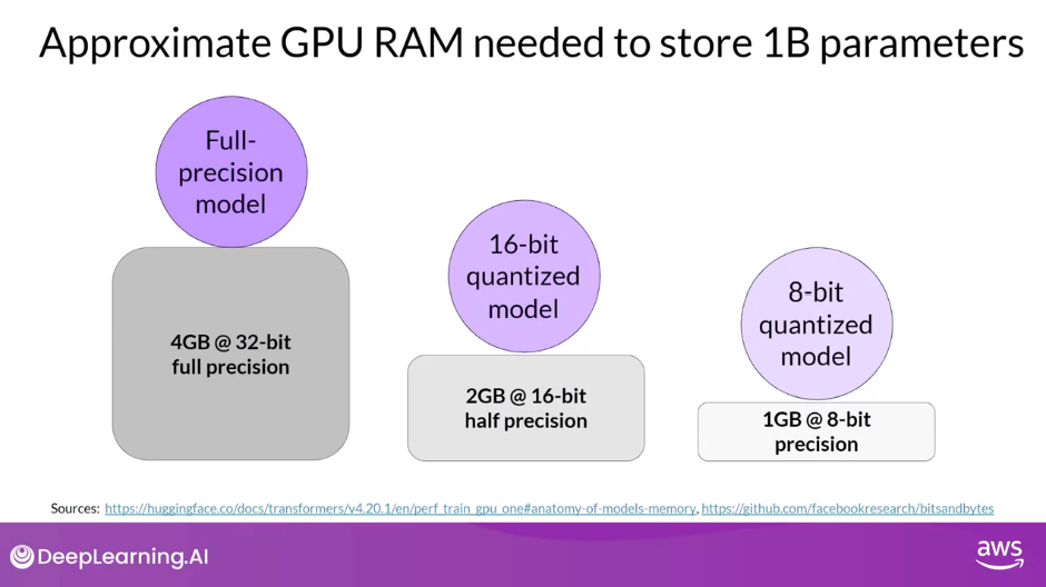
Approximate GPU RAM Needed to Store 1B Parameters #

• A single parameter is typically represented by a 32-bit float, which is a way computers represent real numbers.
• You’ll see more details about how numbers gets stored in this format shortly.
• A 32-bit float takes up four bytes of memory.
• So to store one billion parameters you’ll need four bytes times one billion parameters, or four gigabyte of GPU RAM at 32-bit full precision.
• This is a lot of memory, and note, if only accounted for the memory to store the model weights so far.

Additional GPU RAM Needed to Train 1 B Parameters #

• If you want to train the model, you’ll have to plan for additional components that use GPU memory during training. These include
  1. two Adam optimizer states,
  2. gradients,
  3. activations, and
  4. temporary variables needed by your functions.
• This can easily lead to 20 extra bytes of memory per model parameter.

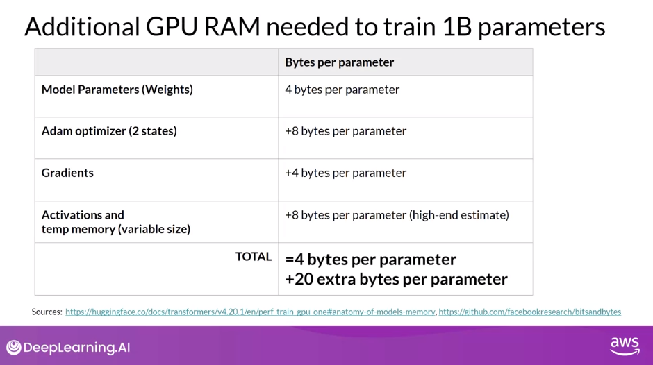
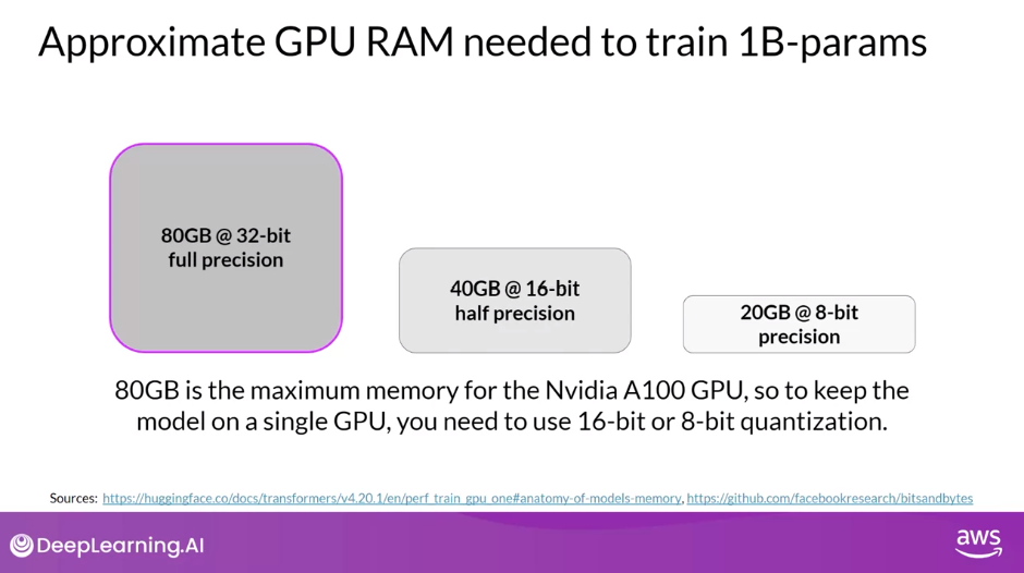
• In fact, to account for all of these overhead during training, you’ll actually require approximately 20 times the amount of GPU RAM that the model weights alone take up.
• To train a one billion parameter model at 32-bit full precision, you’ll need approximately 80 gigabyte of GPU RAM.
• This is definitely too large for consumer hardware, and even challenging for hardware used in data centers, if you want to train with a single processor.
• Eighty gigabyte is the memory capacity of a single NVIDIA A100 GPU, a common processor used for machine learning tasks in the Cloud.

What options do you have to reduce the memory required for training?

• One technique that you can use to reduce the memory is called Quantization.

Quantization #

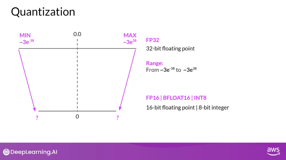
• The main idea here is that you reduce the memory required to store the weights of your model by reducing their precision from 32-bit floating point numbers to 16-bit floating point numbers, or eight-bit integer numbers. The corresponding data types used in deep learning frameworks and libraries are
  • FP32 for 32-bit full position,
  • FP16, or BFLOAT16 for 16-bit half precision, and
  • INT8 eight-bit integers.
• The range of numbers you can represent with FP32 goes from approximately 3x10^-38 to 3x10^38.
• By default, model weights, activations, and other model parameters are stored in FP32.
• Quantization statistically projects the original 32-bit floating point numbers into a lower precision space, using scaling factors calculated based on the range of the original 32-bit floating point numbers.

Quantization: PI in FP32 #

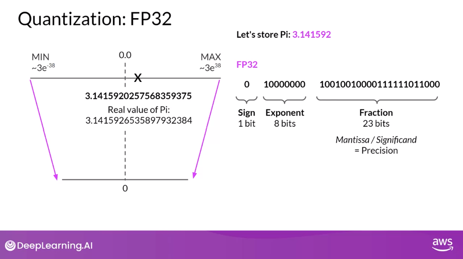
• Suppose you want to store a PI to six decimal places in different positions. Floating point numbers are stored as a series of bits zeros and ones.
• The 32 bits to store numbers in full precision with FP32 consist of
  • one bit for the sign where zero indicates a positive number, and one a negative number. Then
  • eight bits for the exponent of the number, and
  • 23 bits representing the fraction of the number. The fraction is also referred to as the mantissa, or significand. It represents the precision bits off the number.
• If you convert the 32-bit floating point value back to a decimal value, you notice the slight loss in precision. For reference, here’s the real value of PI to 19 decimal places.

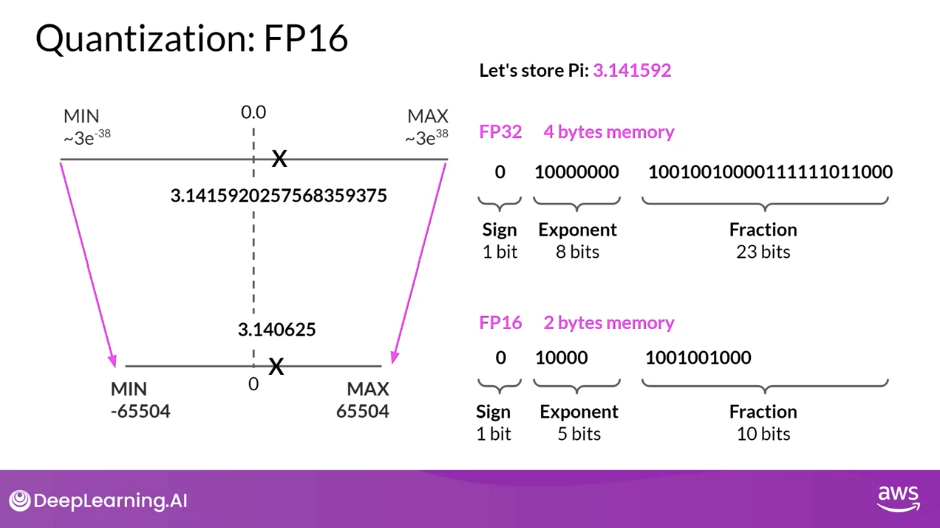
Quantization: FP16 #

• Now, let’s see what happens if you project this FP32 representation of PI into the FP16, 16-bit lower precision space. The 16 bits consists of
  • one bit for the sign, as you saw for FP32, but now FP16 only assigns
  • five bits to represent the exponent and
  • 10 bits to represent the fraction.
• Therefore, the range of numbers you can represent with FP16 is vastly smaller from negative 65,504 to positive 65,504.
• The original FP32 value gets projected to 3.140625 in the 16-bit space.
• Notice that you lose some precision with this projection.
• There are only six places after the decimal point now.
• You’ll find that this loss in precision is acceptable in most cases because you’re trying to optimize for memory footprint.
• Storing a value in FP32 requires four bytes of memory.
• In contrast, storing a value on FP16 requires only two bytes of memory, so with quantization you have reduced the memory requirement by half.

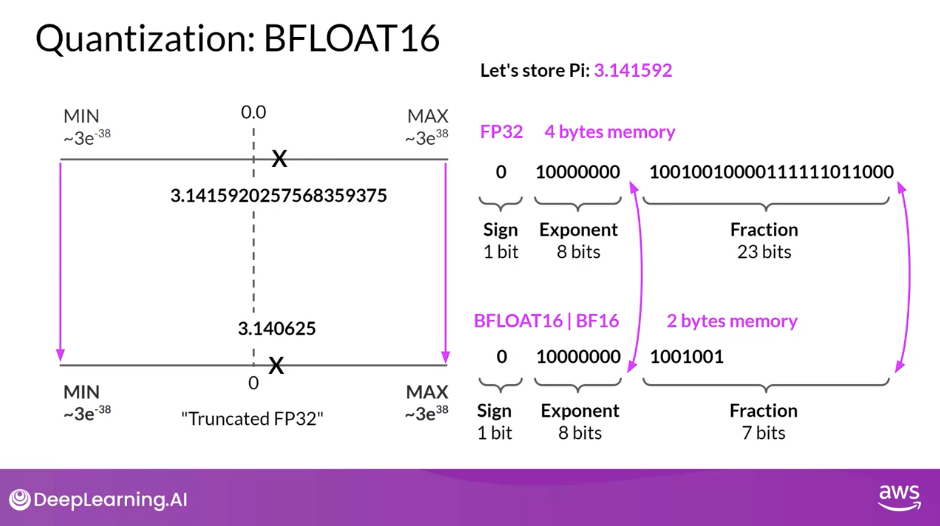
Quantization: BFLOAT16 #

• The AI research community has explored ways to optimize 16-bit quantization.
• One datatype in particular BFLOAT16, has recently become a popular alternative to FP16.
• BFLOAT16, short for Brain Floating Point Format developed at Google Brain has become a popular choice in deep learning.
• Many LLMs, including FLAN-T5, have been pre-trained with BFLOAT16.
• BFLOAT16 or BF16 is a hybrid between half precision FP16 and full precision FP32.
• BF16 significantly helps with training stability and is supported by newer GPU’s such as NVIDIA’s A100.
• BFLOAT16 is often described as a truncated 32-bit float, as it captures the full dynamic range of the full 32-bit float, that uses only 16-bits.
• BFLOAT16 uses the full eight bits to represent the exponent, but truncates the fraction to just seven bits.
• This not only saves memory, but also increases model performance by speeding up calculations.
• The downside is that BF16 is not well suited for integer calculations, but these are relatively rare in deep learning.

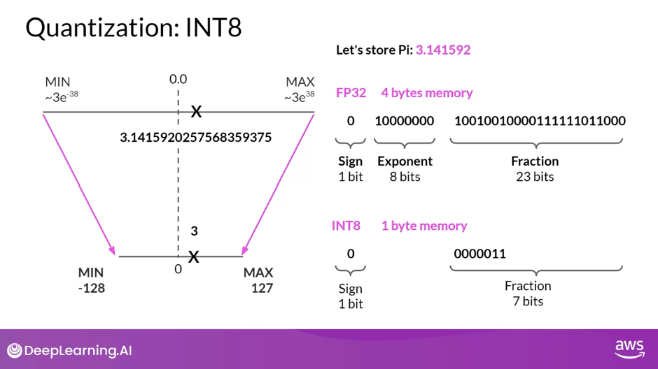
Quantization: INT8 #

• For completeness let’s have a look at what happens if you quantize PI from the 32-bit into the even lower precision eight bit space. If you use
  • one bit for the sign INT8
  • values are represented by the remaining seven bits.
• This gives you a range to represent numbers from negative 128 to positive 127 and unsurprisingly PI gets projected two or three in the 8-bit lower precision space.
• This brings new memory requirement down from originally four bytes to just one byte, but obviously results in a pretty dramatic loss of precision.

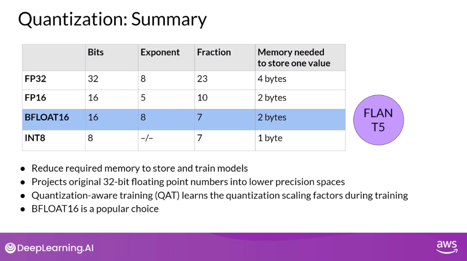
Quantization: Summary #

• Remember that the goal of quantization is to reduce the memory required to store and train models by reducing the precision off the model weights.
• Quantization statistically projects the original 32-bit floating point numbers into lower precision spaces using scaling factors calculated based on the range of the original 32-bit floats.
• Modern deep learning frameworks and libraries support Quantization-Aware Training (QAT), which learns the quantization scaling factors during the training process. The details of this process are beyond the scope of this course.
• But you’ve seen the key point here, that you can use quantization to reduce the memory footprint off the model during training.
• BFLOAT16 has become a popular choice of precision in deep learning as it maintains the dynamic range of FP32, but reduces the memory footprint by half.
• Many LLMs, including FLAN-T5, have been pre-trained with BFOLAT16.

Visualization: Quantization #

• Let’s return to the challenge of fitting models into GPU memory and take a look at the impact quantization can have
• By applying quantization, you can reduce your memory consumption required to store the model parameters down to only two gigabyte using 16-bit half precision of 50% saving and you could further reduce the memory footprint by another 50% by representing the model parameters as eight bit integers, which requires only one gigabyte of GPU RAM.
• Note that in all these cases you still have a model with one billion parameters. As you can see, the circles representing the models are the same size

• Quantization will give you the same degree of savings when it comes to training.
• As you heard earlier, you’ll quickly hit the limit of a single NVIDIA A100 GPU with 80 gigabytes of memory, when you try to train a one billion parameter model at 32-bit full precision.
• You’ll need to consider using either 16-bit or eight bit quantization if you want to train on a single GPU

GPU RAM Needed to Train Larger Models #

• Remember, many models now have sizes in excess of 50 billion or even 100 billion parameters, meaning you’d need up to 500 times more memory capacity to train them, tens of thousands of gigabytes.
• These enormous models dwarf the one billion parameter model we’ve been considering, shown here to scale on the left

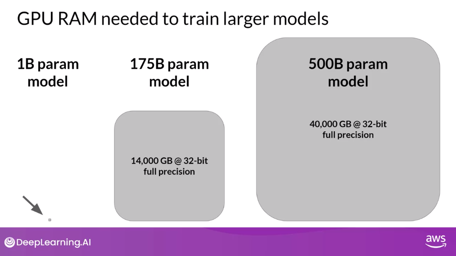
• As models scale beyond a few billion parameters, it becomes impossible to train them on a single GPU.
• Instead, you’ll need to turn to distributed computing techniques while you train your model across multiple GPUs.
• This could require access to hundreds of GPUs, which is very expensive, another reason why you won’t pre-train your own model from scratch most of the time

• However, an additional training process called Fine-tuning also require storing all training parameters in memory and it’s very likely you’ll want to fine tune a model at some point.

Optional: Efficient Multi-GPU Compute Strategies #

• Need to scale your model training efforts beyond a single GPU.
• Need to use multi GPU compute strategies when your model becomes too big to fit in a single GPU
• But even if your model does fit onto a single GPU, there are benefits to using multiple GPUs to speed up your training
• It’s useful to know how to distribute compute across GPUs even when you’re working with a small model

Let’s discuss how you can carry out this scaling across multiple GPUs in an efficient way.

Distributed Data Parallel (DDP) #

Model still fits on a single GPU

• The first step in scaling model training is to distribute large data-sets across multiple GPUs and process these batches of data in parallel.
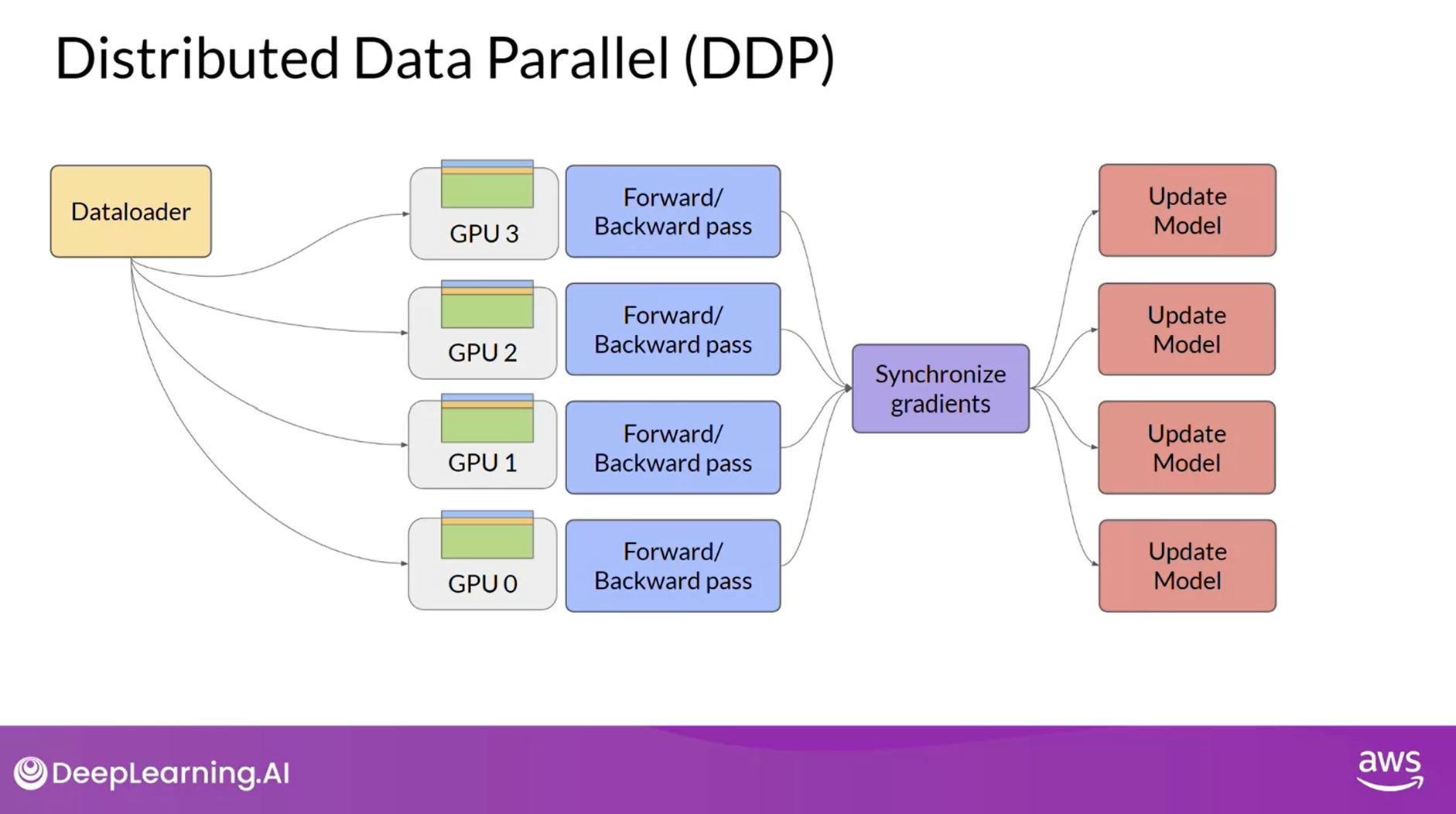
• A popular implementation of this model replication technique is PyTorch’s Distributed Data Parallel (DDP)
  • DDP copies your model onto each GPU and sends batches of data to each of the GPUs in parallel.
  • Each data-set is processed in parallel and then a synchronization step combines the results of each GPU, which in turn updates the model on each GPU, which is always identical across chips.
  • This implementation allows parallel computations across all GPUs that results in faster training.
• Note: DDP requires that your model weights and all of the additional parameters, gradients, and optimizer states that are needed for training, fit onto a single GPU.

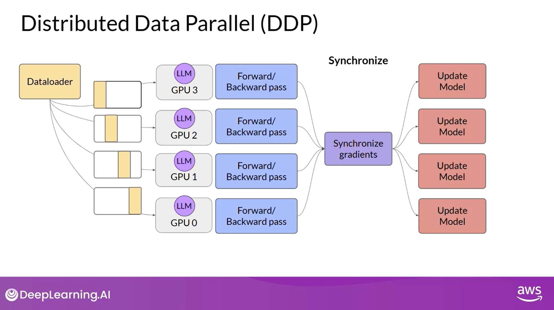
• If your model is too big for this, you should look into another technique called Model Sharding.

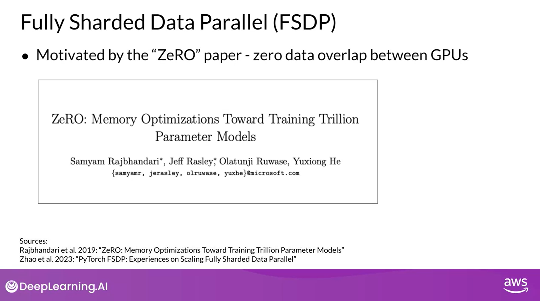
Fully Sharded Data Parallel (FSDP) #

Model no longer fits on a single GPU

• A popular implementation of modal sharding is PyTorch’s Fully Sharded Data Parallel (FSDP)
• FSDP is motivated by a paper published by researchers at Microsoft in 2019 that proposed a technique called ZeRO.
• ZeRO stands for Zero Redundancy Optimizer and the goal of ZeRO is to optimize memory by distributing or sharding model states across GPUs with ZeRO data overlap.
  • This allows you to scale model training across GPUs when your model doesn’t fit in the memory of a single chip.

Let’s take a quick look at how ZeRO works before coming back to FSDP.

• Looked at all of the memory components required for training LLMs, the largest memory requirement was for
  1. the optimizer states, which take up twice as much space as the weights, followed by
  2. weights themselves and
  3. the gradients.

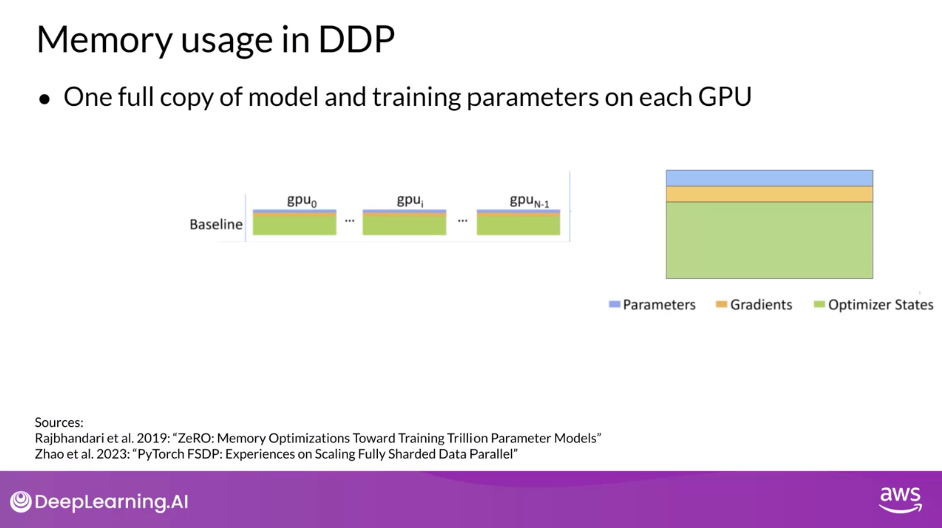
Memory Usage in DDP #

• Let’s represent the parameters as this blue box, the gradients and yellow and the optimizer states in green.
• One limitation off the model replication strategy that I showed before is that you need to keep a full model copy on each GPU, which leads to redundant memory consumption. You are storing the same numbers on every GPU.

Zero Redundancy Optimizer #

• ZeRO, on the other hand, eliminates this redundancy by distributing also referred to as sharding the model parameters, gradients, and optimizer states across GPUs instead of replicating them.
• At the same time, the communication overhead for a sinking model states stays close to that of the previously discussed DDP.
• ZeRO offers three optimization stages.
  • ZeRO Stage 1, shots only optimizer states across GPUs, this can reduce your memory footprint by up to a factor of four.
  • ZeRO Stage 2 also shots the gradients across chips. When applied together with Stage 1, this can reduce your memory footprint by up to eight times.
  • Finally, ZeRO Stage 3 shots all components including the model parameters across GPUs.
• When applied together with Stages 1 and 2, memory reduction is linear with a number of GPUs.
  • For example, sharding across 64 GPUs could reduce your memory by a factor of 64.

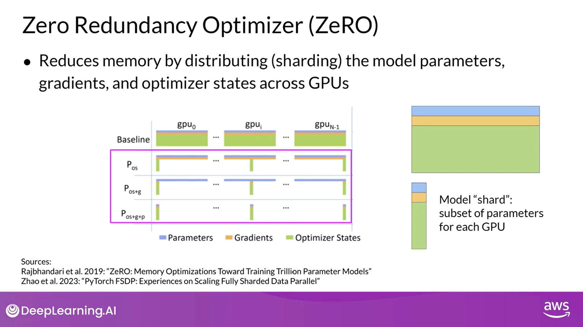
Let’s apply this concept to the visualization of DDP and replace the LLM by the memory representation of model parameters, gradients, and optimizer states.

Visualization: Distributed Data Parallel #

Visualization: Fully Sharded Data Parallel #

• When you use FSDP, you distribute the data across multiple GPUs as you saw happening in DDP.
• But with FSDP, you also distributed or shard the model parameters, gradients, and optimize the states across the GPU nodes using one of the strategies specified in the ZeRO paper.
• With this strategy, you can now work with models that are too big to fit on a single chip.

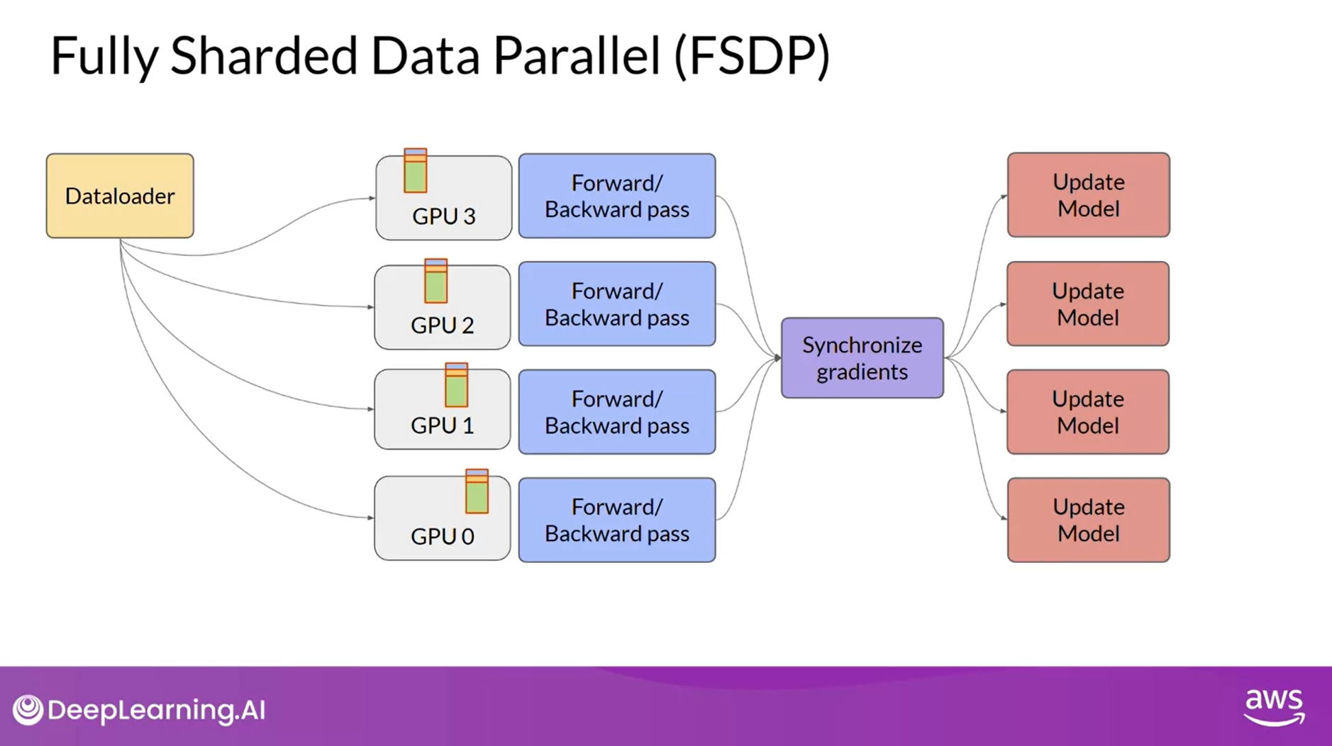
• In contrast to GDP, where each GPU has all of the model states required for processing each batch of data available locally, FSDP requires you to collect this data from all of the GPUs before the forward and backward pass.
• Each CPU requests data from the other GPUs on-demand to materialize the sharded data into uncharted data for the duration of the operation.
• After the operation, you release the uncharted non-local data back to the other GPUs as original sharded data You can also choose to keep it for future operations during backward pass for example.
• Note, this requires more GPU RAM again, this is a typical performance versus memory trade-off decision.

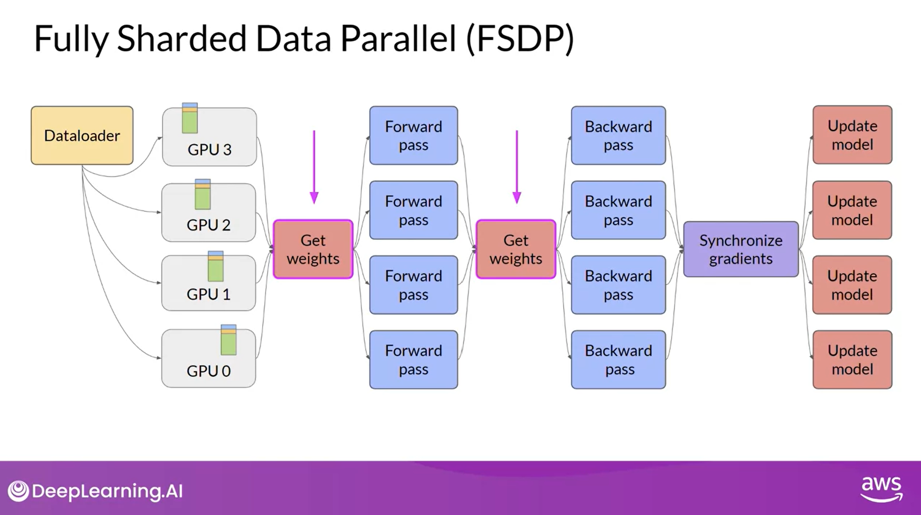
• In the final step after the backward pass, FSDP is synchronizes the gradients across the GPUs in the same way they were for DDP.

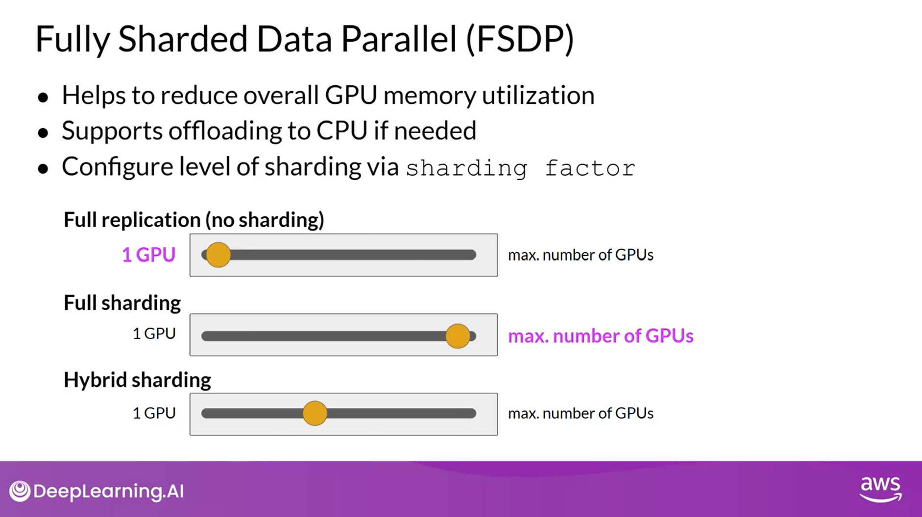
Sharding Factor #

• Model Sharding as described with FSDP allows you to reduce your overall GPU memory utilization.
• Optionally, you can specify that FSDP offloads part of the training computation to GPUs to further reduce your GPU memory utilization.
• To manage the trade-off between performance and memory utilization, you can configure the level of sharding using FSDP is sharding factor.
  • A sharding factor of one basically removes the sharding and replicates the full model similar to DDP.
  • If you set the sharding factor to the maximum number of available GPUs, you turn on full sharding.
    • This has the most memory savings, but increases the communication volume between GPUs.
  • Any sharding factor in-between enables hybrid sharding.

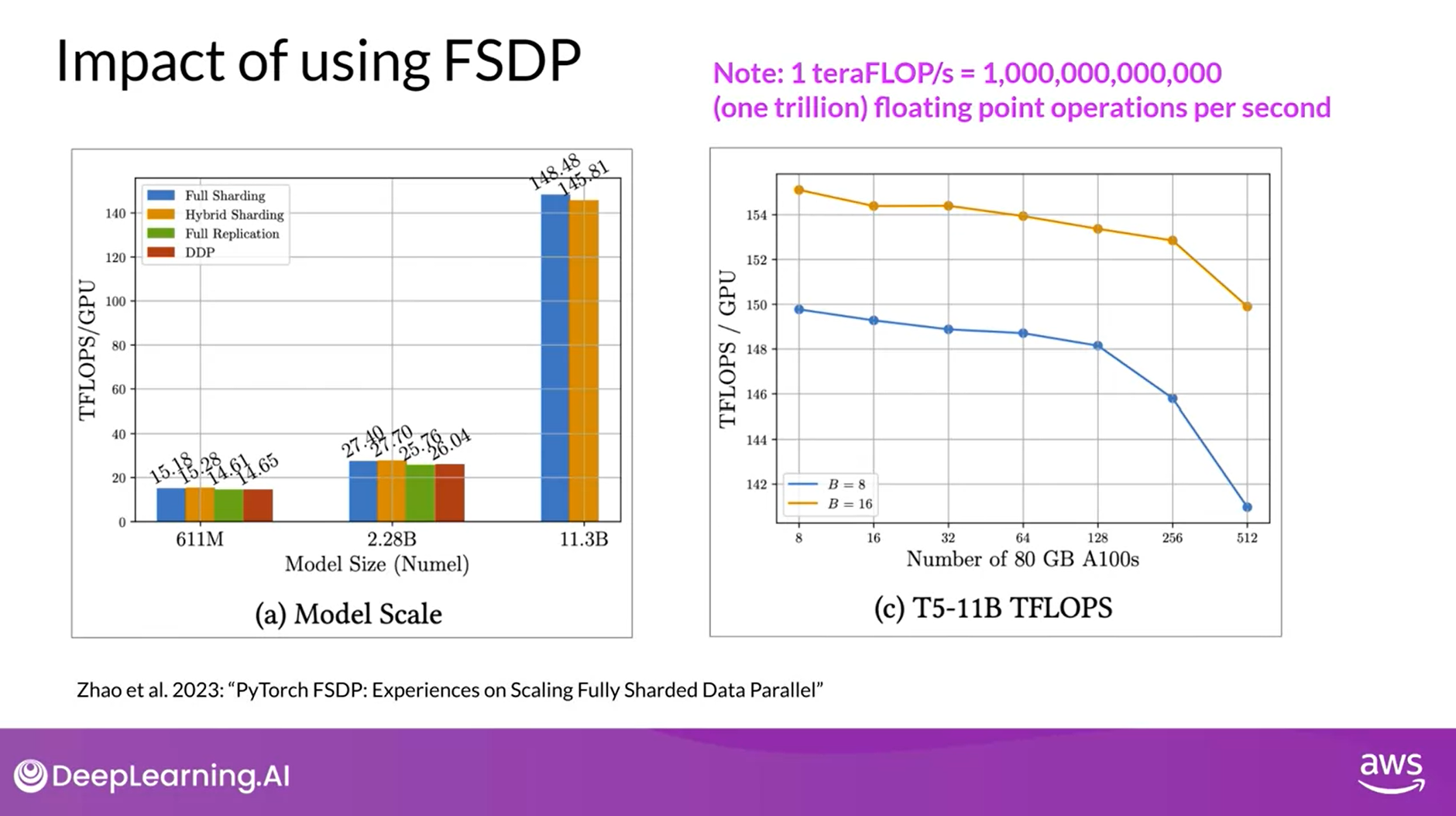
Impact of Using FSDP #

• Let’s take a look at how FSDP performs in comparison to DDP measured in teraflops per GPU.
• These tests were performed using a maximum of 512 NVIDIA V100 GPUs, each with 80 gigabytes of memory.
• Note, one teraflop corresponds to one trillion floating-point operations per second.
• The first figure shows FSDP performance for different size T5 models.
  • You can see the different performance numbers for FSDP, full sharding in blue, hybrid shard in orange and full replication in green.
  • For reference, DDP performance is shown in red.
  • For the first 25 models with 611 million parameters and 2.28 billion parameters, the performance of FSDP and DDP is similar.
  • Now, if you choose a model size beyond 2.28 billion, such as T5 with 11.3 billion parameters, DDP runs into the out-of-memory error.
  • FSDP on the other hand can easily handle models this size and achieve much higher teraflops when lowering the model’s precision to 16-bit.
• The second figure shows 7% decrease in per GPU teraflops when increasing the number of GPUs from 8-512 for the 11 billion T5 model, plotted here using a batch size of 16 and orange and a batch size of eight in blue.
  • As the model grows in size and is distributed across more and more GPUs, the increase in communication volume between chips starts to impact the performance, slowing down the computation.
• In summary, this shows that you can use FSDP for both small and large models and seamlessly scale your model training across multiple GPUs.

• The most important thing is to have a sense of how the data model parameters and training computations are shared across processes when training LLMs.
• Given the expense and technical complexity of training models across GPUs, some researchers have been exploring ways to achieve better performance with smaller models.

Question: Which of the following best describes the role of data parallelism in the context of training Large Language Models (LLMs) with GPUs?

Data parallelism allows for the use of multiple GPUs to process different parts of the same data simultaneously, speeding up training time.

Correct Data parallelism is a strategy that splits the training data across multiple GPUs. Each GPU processes a different subset of the data simultaneously, which can greatly speed up the overall training time.

Scaling Laws and Compute-Optimal Methods #

• Learn about research that has explored the relationship between

  • model size,
  • training,
  • configuration and
  • performance

  in an effort to determine just how big models need to be

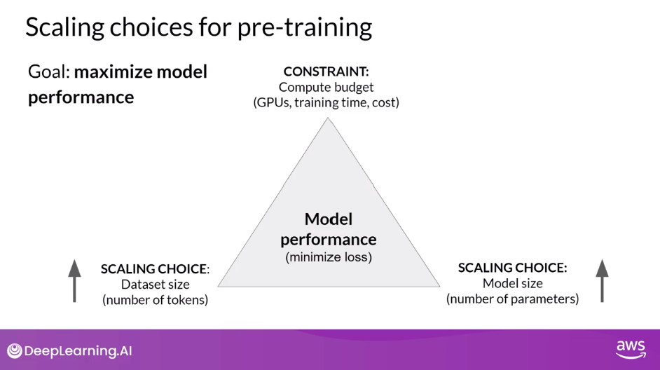
Scaling Choices for Pre-training #

• Remember, the goal during pre-training is to maximize the model’s performance of its learning objective, which is minimizing the loss when predicting tokens.
• Two options you have to achieve better performance are
  1. increasing the size of the dataset you train your model on and
  2. increasing the number of parameters in your model.
  • In theory, you could scale either of both of these quantities to improve performance.
• However, another issue to take into consideration is
  • your compute budget which includes factors like the number of GPUs you have access to and
  • the time you have available for training models

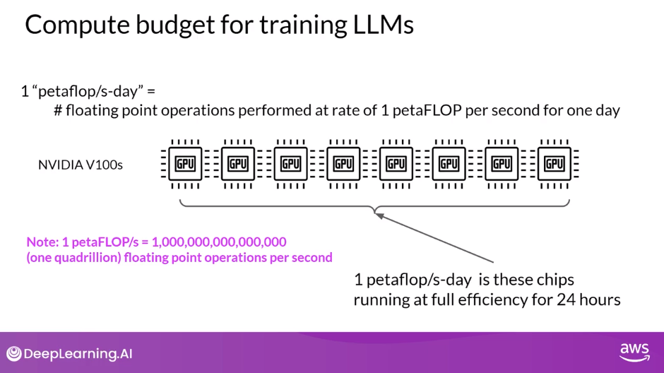
Unit of Compute #

• To help you understand some of the discussion ahead, let’s first define a unit of compute that quantifies the required resources.
• A petaFLOP per second-day is a measurement of the number of floating point operations performed at a rate of one petaFLOP per second, running for an entire day.
• Note: one petaFLOP corresponds to one quadrillion floating point operations per second.
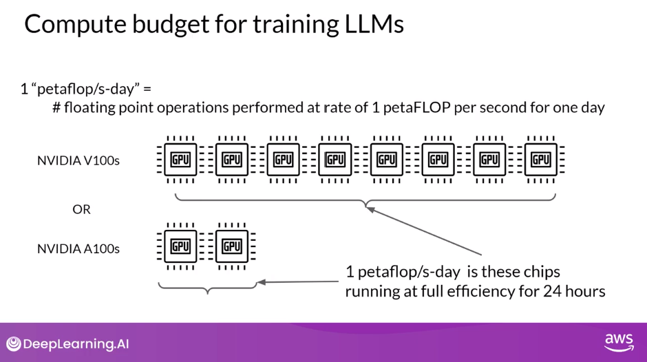
• When specifically thinking about training transformers, one petaFLOP per second day is approximately equivalent to eight NVIDIA V100 GPUs, operating at full efficiency for one full day.

• If you have a more powerful processor that can carry out more operations at once, then a petaFLOP per second day requires fewer chips.
  • For example, two NVIDIA A100 GPUs give equivalent compute to the eight V100 chips.

Number of PetaFLOP/s-days to Pre-train Various LLMs #

• To give you an idea off the scale of these compute budgets, this chart shows a comparison off the petaFLOP per second days required to pre-train different variants of
  • BERT and RoBERTa, which are both encoder only models,
  • T5 and encoder-decoder model and
  • GPT-3, which is a decoder only model.
• The difference between the models in each family is the number of parameters that were trained, ranging from a few hundred million for BERT base to 175 billion for the largest GPT-3 variant.
• Note that the y-axis is logarithmic. Each increment vertically is a power of 10.
• Here we see that T5 XL with three billion parameters required close to 100 petaFLOP per second days while the larger GPT-3 175 billion parameter model required approximately 3,700 petaFLOP per second days.
• This chart makes it clear that a huge amount of computers required to train the largest models.

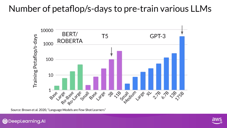
• You can see that bigger models take more compute resources to train and generally also require more data to achieve good performance.
• It turns out that they are actually well-defined relationships between these three scaling choices.

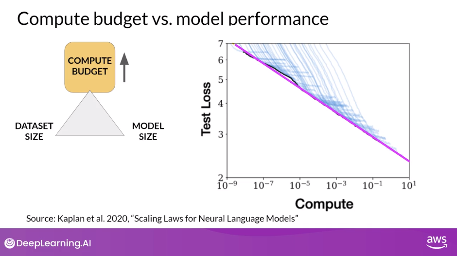
Compute Budget vs Model Performance #

• Researchers have explored the trade-offs between training dataset size, model size and compute budget. Here’s a figure from a paper by researchers at OpenAI that explores the impact of compute budget on model performance.
  • The y-axis is the test loss, which you can consider as a proxy for model performance where smaller values are better.
  • The x-axis is the compute budget in units of petaFLOP per second days.
• As you just saw, larger numbers can be achieved by either using more compute power or training for longer or both.
• Each thin blue line here shows the model loss over a single training run. Looking at where the loss starts to decline more slowly for each run, reveals a clear relationship between the compute budget and the model’s performance.
• This can be approximated by a power-law relationship, shown by this pink line.
• A power law is a mathematical relationship between two variables, where one is proportional to the other raised to some power.
• When plotted on a graph where both axes are logarithmic, power-law relationships appear as straight lines.
• The relationship here holds as long as model size and training dataset size don’t inhibit the training process.
• Taken at face value, this would suggest that you can just increase your compute budget to achieve better model performance.

Dataset Size and Model Size vs Performance #

• In practice however, the compute resources you have available for training will generally be a hard constraint set by factors such as
  • the hardware you have access to,
  • the time available for training and
  • the financial budget of the project.
• If you hold your compute budget fixed, the two levers you have to improve your model’s performance are
  • the size of the training dataset and
  • the number of parameters in your model
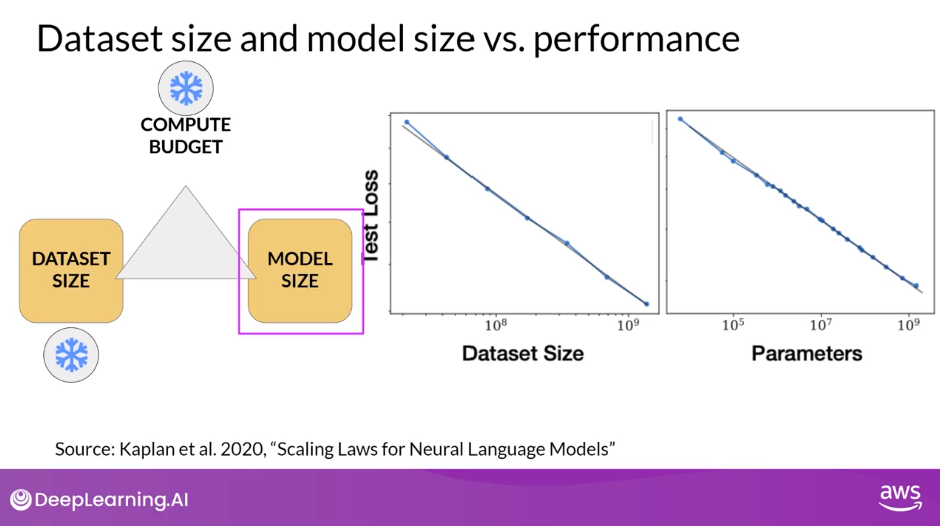
• The OpenAI researchers found that these two quantities also show a power-law relationship with a test loss in the case where the other two variables are held fixed

• This is another figure from the paper exploring the impact of training dataset size on model performance.
  • Here, the compute budget and model size are held fixed and the size of the training dataset is vary.
  • The graph shows that as the volume of training data increases, the performance of the model continues to improve.
• In the second graph, the compute budget and training dataset size are held constant. Models of varying numbers of parameters are trained.
  • As the model increases in size, the test loss decreases indicating better performance.

• At this point you might be asking, what’s the ideal balance between these three quantities?
• Well, it turns out a lot of people are interested in this question.
• Both research and industry communities have published a lot of empirical data for pre-training compute optimal models

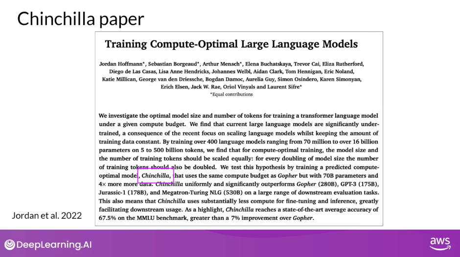
Chinchilla Paper: Training Compute-Optimal Large Language Models #

• In a paper published in 2022, a group of researchers led by Jordan Hoffmann, Sebastian Borgeaud and Arthur Mensch carried out a detailed study of the performance of language models of various sizes and quantities of training data.
• The goal was to find the optimal number of parameters and volume of training data for a given compute budget. The authors name the resulting compute optimal model, Chinchilla.
• This paper is often referred to as the Chinchilla paper.

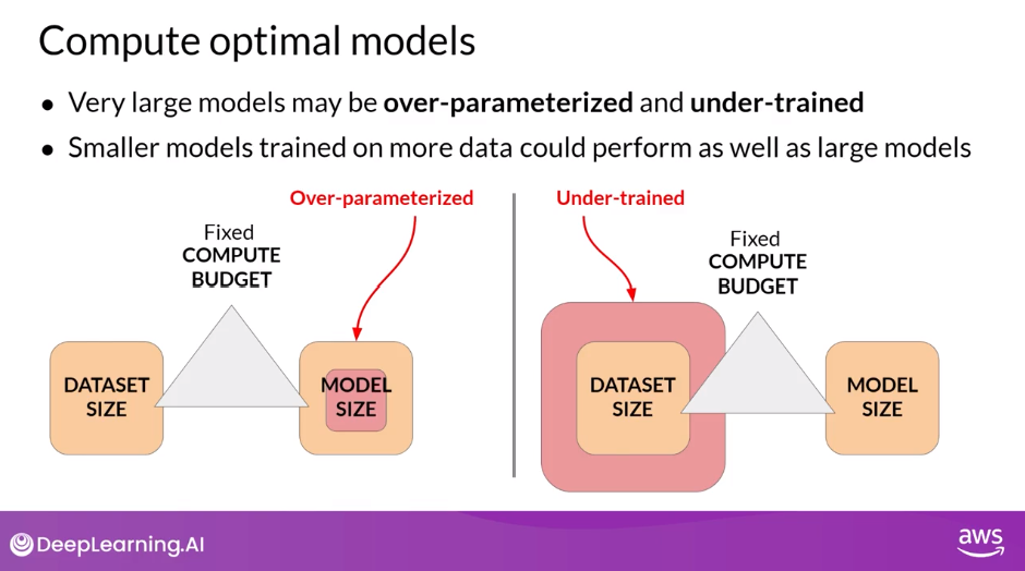
Compute Optimal Models #

• The Chinchilla paper hints that many of the 100 billion parameter large language models like GPT-3 may actually be over-parameterized, meaning they have more parameters than they need to achieve a good understanding of language and under-trained so that they would benefit from seeing more training data.
• The authors hypothesized that smaller models may be able to achieve the same performance as much larger ones if they are trained on larger datasets

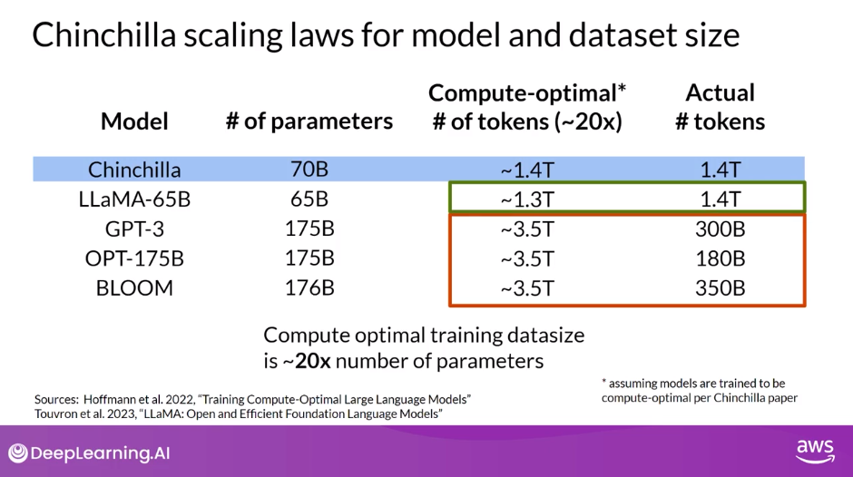
Chinchilla Scaling Laws for Model and Dataset Size #

• In this table, you can see a selection of models along with their size and information about the dataset they were trained on.
• One important takeaway from the Chinchilla paper is that the optimal training dataset size for a given model is about 20 times larger than the number of parameters in the model.
• Chinchilla was determined to be compute optimal.
  • For a 70 billion parameter model, the ideal training dataset contains 1.4 trillion tokens or 20 times the number of parameters.
• The last three models in the table were trained on datasets that are smaller than the Chinchilla optimal size. These models may actually be under trained.
• In contrast, LLaMA was trained on a dataset size of 1.4 trillion tokens, which is close to the Chinchilla recommended number.
• Another important result from the paper is that the compute optimal Chinchilla model outperforms non-compute optimal models such as GPT-3 on a large range of downstream evaluation tasks

Model Size vs Time #

• With the results of the Chinchilla paper in hand teams have recently started to develop smaller models that achieved similar, if not better results than larger models that were trained in a non-optimal way.
• Moving forward, you can probably expect to see a deviation from the bigger is always better trends of the last few years as more teams or developers like you start to optimize their model design.
• The last model shown on this slide, BloombergGPT, is a really interesting model.
  • It was trained in a compute optimal way following the Chinchilla loss and so achieves good performance with the size of 50 billion parameters

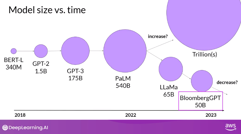
It’s also an interesting example of a situation where pre-training a model from scratch was necessary to achieve good task performance.

Pre-training for Domain Adaptation #

• If your target domain uses vocabulary and language structures that are not commonly used in day to day language, you may need to perform domain adaptation to achieve good model performance.

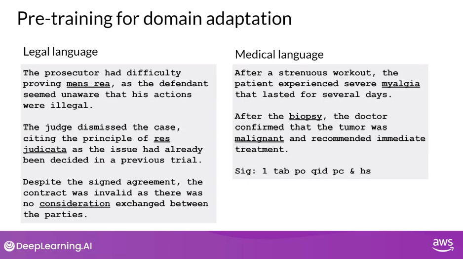
Legal Language #

• For example, imagine you’re a developer building an app to help lawyers and paralegals summarize legal briefs. Legal writing makes use of very specific terms like mens rea in the first example and res judicata in the second.
• These words are rarely used outside of the legal world, which means that they are unlikely to have appeared widely in the training text of existing LLMs. As a result, the models may have difficulty understanding these terms or using them correctly.
• Another issue is that legal language sometimes uses everyday words in a different context, like consideration in the third example. Which has nothing to do with being nice, but instead refers to the main element of a contract that makes the agreement enforceable.

Medical Language #

• For similar reasons, you may face challenges if you try to use an existing LLM in a medical application. Medical language contains many uncommon words to describe medical conditions and procedures. And these may not appear frequently in training datasets consisting of web scrapes and book texts. Some domains also use language in a highly idiosyncratic way.
• This last example of medical language may just look like a string of random characters, but it’s actually a shorthand used by doctors to write prescriptions. This text has a very clear meaning to a pharmacist, take one tablet by mouth four times a day, after meals and at bedtime

• Because models learn their vocabulary and understanding of language through the original pretraining task.
• Pretraining your model from scratch will result in better models for highly specialized domains like law, medicine, finance or science

BloombergGPT: Domain Adapatation for Finance #

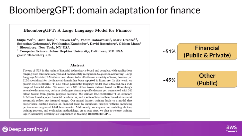
• First announced in 2023 in a paper by Shijie Wu, Steven Lu, and colleagues at Bloomberg
• BloombergGPT is an example of a large language model that has been pretrained for a specific domain, in this case, finance
• The Bloomberg researchers chose to combine both finance data and general purpose tax data to pretrain a model that achieves best in class results on financial benchmarks, while also maintaining competitive performance on general purpose LLM benchmarks.
  • As such, the researchers chose data consisting of 51% financial data and 49% public data.
• In their paper, the Bloomberg researchers describe the model architecture in more detail.
• They also discuss how they started with a Chinchilla Scaling Laws for guidance and where they had to make tradeoffs

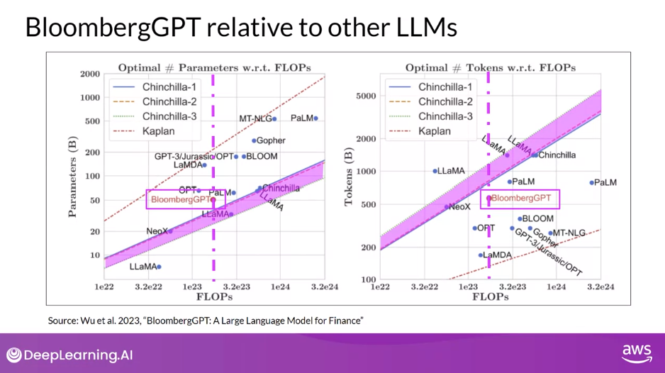
Scaling Laws #

• These two graphs compare a number of LLMs, including BloombergGPT, to scaling laws that have been discussed by researchers.
  • On the left, the diagonal lines trace the optimal model size in billions of parameters for a range of compute budgets.
  • On the right, the lines trace the compute optimal training data set size measured in number of tokens.
• The dashed pink line on each graph indicates the compute budget that the Bloomberg team had available for training their new model.
• The pink shaded regions correspond to the compute optimal scaling loss determined in the Chinchilla paper.
• In terms of model size, you can see that BloombergGPT roughly follows the Chinchilla approach for the given compute budget of 1.3 million GPU hours, or roughly 230,000,000 petaflops.
• The model is only a little bit above the pink shaded region, suggesting the number of parameters is fairly close to optimal.
• However, the actual number of tokens used to pretrain BloombergGPT 569,000,000,000 is below the recommended Chinchilla value for the available compute budget.
• The smaller than optimal training data set is due to the limited availability of financial domain data showing that real world constraints may force you to make trade offs when pretraining your own models

Key Takeways #

• Walked you through some of the common use cases for LLMs, such as essay writing, dialogue summarization and translation.
• Gave a detailed presentation of the transformer architecture that powers these models.
• Discussed some of the parameters you can use at inference time to influence the model’s output.
• Introduced to Generative AI Project Lifecycle that you can use to plan and guide your application development work.
• Saw how models are trained on vast amounts of text data during an initial training phase called pretraining. This is where models develop their understanding of language.
• Explored some of the computational challenges of training these models, which are significant. In practice, because of GPU memory limitations, you will almost always use some form of quantization when training your models.
• Finished with a discussion of scaling laws that have been discovered for LLMs and how they can be used to design compute optimal models.

Question: Which of the following statements about pretraining scaling laws are correct? Select all that apply:

Which of the following statements about pretraining scaling laws are correct? Select all that apply:

To scale our model, we need to jointly increase dataset size and model size, or they can become a bottleneck for each other.

Correct

For instance, while increasing dataset size is helpful, if we do not jointly improve the model size, it might not be able to capture value from the larger dataset.

There is a relationship between model size (in number of parameters) and the optimal number of tokens to train the model with.

Correct

This relationship is describe in the Chinchilla paper, that shows that many models might even be overparametrized according to the relationship they found.

When measuring compute budget, we can use “PetaFlops per second-Day” as a metric.

Correct

Petaflops per second-day is a useful measure for computing budget as it reflects the both hardware and time required to train the model.

Reading: Domain-Specific Training: BloombergGPT #

• BloombergGPT - https://arxiv.org/abs/2303.17564
  • a large Decoder-only language model
  • underwent pre-training using an extensive financial dataset to increase its understanding of finance and enabling it to generate finance-related natural language text.
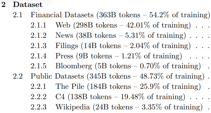
    • Dataset comprises of
      • news articles
      • reports
      • market data
  • During the training of BloombergGPT, the authors used the Chinchilla Scaling Laws to guide the number of parameters in the model and the volume of training data, measured in tokens.
  • The recommendations of Chinchilla are represented by the lines Chinchilla-1, Chinchilla-2 and Chinchilla-3 in the image, and we can see that BloombergGPT is close to it.
  • While the recommended configuration for the team’s available training compute budget was 50 billion parameters and 1.4 trillion tokens, acquiring 1.4 trillion tokens of training data in the finance domain proved challenging.
  • Consequently, they constructed a dataset containing just 700 billion tokens, less than the compute-optimal value. Furthermore, due to early stopping, the training process terminated after processing 569 billion tokens.
  • The BloombergGPT project is a good illustration of pre-training a model for increased domain-specificity, and the challenges that may force trade-offs against compute-optimal model and training configurations.